Getting the variables of interest

We can get the variables we are interested in by extracting the disp and mpg columns of the data.

disp = cars2020[["disp"]]
mpg = cars2020[["mpg"]]

An exploratory scatter plot

Next, I made an exploratory scatter plot of the relationship between the two variables, using matplotlib.pyplot

import matplotlib.pyplot as plt
plt.scatter(disp, mpg, alpha = 0.25)
plt.title("MPG vs engine displacement", fontdict={'fontsize': 6, 'fontweight': 'medium'})
plt.show()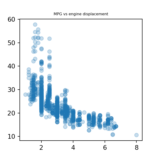

Modeling

To carry out the actual linear regression, we use the scikit-learn library.

• Import linear_model
• Instantiate an object of type LinearRegression

from sklearn import linear_model
regr = linear_model.LinearRegression()
type(regr)

<class 'sklearn.linear_model._base.LinearRegression'>

Next fit the model with the vectors of predictors (X) and outcomes (Y)

regr.fit(disp, mpg)

LinearRegression(copy_X=True, fit_intercept=True, n_jobs=None, normalize=False)

The above function call causes the intercept_ and coef_ properties of regr to be the intercept and slope terms of the model.

We can print the values of the model parameters:

print("Model 1\n", "Intercept: ", regr.intercept_,"\nCoefficients", regr.coef_)

Model 1
 Intercept:  [34.05220566] 
Coefficients [[-3.4131261]]

Showing the regression line

The code below manually superimposes the regression line onto the scatter plot of mpg vs displacement

plt.scatter(disp, mpg, alpha = 0.2)
plt.plot([0,8], [regr.intercept_, regr.coef_*8 + regr.intercept_], "--", color = "red")
plt.title("MPG vs engine displacement", fontdict={'fontsize': 6, 'fontweight': 'medium'})
plt.show()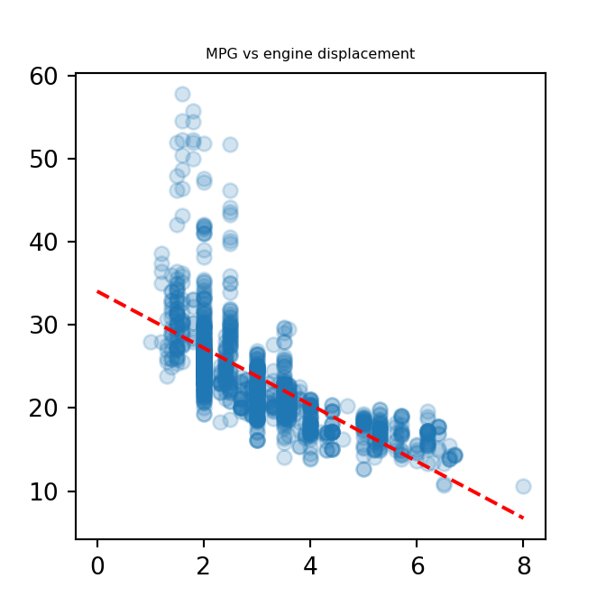

Getting the model predicted values

We can use the predict method of the LinearRegression class to return the vector of model outputs for each element of the input vector, disp

model1_mpg = regr.predict(disp)

Plotting model vs actual

One way to compare the model predicted values to the actual values is to plot them against each other in a scatter plot.

plt.scatter(mpg, model1_mpg, alpha = 0.2)
plt.title("Model MPG vs Actual MPG (model: mpg~disp)", fontdict={'fontsize': 6, 'fontweight': 'medium'})
plt.show()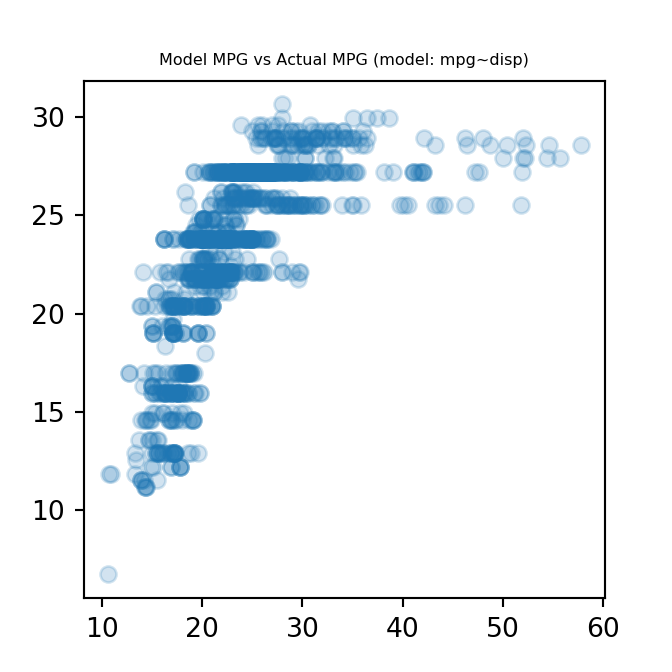

We can modify the above plot by adding a diagonal line with intercept, 0, and slope, 1. A point lying on this line would indicate that the value predicted by the model and the actual value were equal. A model that fits the data closely, would thus have a scatter plot in which the points were typically close to the diagonal line.

plt.scatter(mpg, model1_mpg, alpha = 0.2)
plt.plot([0,60], [0,60], "--", color = "red")
plt.title("Model MPG vs Actual MPG (model: mpg~disp)", fontdict={'fontsize': 6, 'fontweight': 'medium'})
plt.show()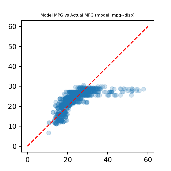

Here we can see that the model does not do as well to predict the vehicles with high fuel-efficiency. Next, I will try to run a multiple linear regression model, with three additional variables, to perhaps get a better model fit.

Creating dummy variables

As some of these variables are categorical, we first have to create dummy variables before fitting the model:

cars_vars = pd.get_dummies(cars_vars, drop_first=True)
cars_vars.head()

   disp  transmission_CVT  ...  atvType_None  atvType_Plug-in Hybrid
0   2.4                 0  ...             1                       0
1   3.5                 0  ...             1                       0
2   3.5                 0  ...             1                       0
3   3.5                 0  ...             1                       0
4   3.0                 0  ...             0                       0

[5 rows x 11 columns]

If the drop_first argument had not been set to True there would be a dummy variable created for each level of each categorical variable. This is not necessary: it suffices to use one level as a reference level and to indicate only if a subject vehicle belongs to any of the other levels.

As it stands, with drop_first=True, dummy variables are created for all but one level of each categorical variable.

Fitting the multiple linear regression model

A call to LinearRegression.fit with the predictors and output data will perform the linear regression

regr_2 = linear_model.LinearRegression()
regr_2.fit(cars_vars, mpg)

LinearRegression(copy_X=True, fit_intercept=True, n_jobs=None, normalize=False)

The model coefficients are now stored in the intercept_ and coef_ properties of the regr_2 object.

Viewing model parameters in multiple linear regression

As before, we can view the model-fitted parameters:

print("Model 2\n", "Intercept: ", regr_2.intercept_,"\nCoefficients", regr_2.coef_)

Model 2
 Intercept:  [30.36387263] 
Coefficients [[-2.37613998  5.07512162  0.72912462  0.3598029   4.85016323  0.13808905
   1.31936111 -2.59373099  4.50478963 -2.5394815   1.63706936]]

model_params = zip(cars_vars.columns, regr_2.coef_[0])

print("Intercept: ", regr_2.intercept_[0])

Intercept:  30.363872634275147

for param in model_params:
  print(param[0], ":", param[1])

disp : -2.376139975429364
transmission_CVT : 5.075121623348058
transmission_Manual : 0.7291246234166626
drive_AWD : 0.3598029024265794
drive_FWD : 4.850163234058179
drive_PT 4WD : 0.13808904559734075
drive_RWD : 1.3193611105192886
atvType_FFV : -2.5937309931581316
atvType_Hybrid : 4.504789629801591
atvType_None : -2.539481497779101
atvType_Plug-in Hybrid : 1.6370693619393155

Retrieving model-predicted values

Now use LinearRegression.predict to get the model-predicted values for each vehicle in the training data.

model2_mpg = regr_2.predict(cars_vars)

Plotting model vs actual values

And once again, use matplotlib.pyplot to plot the model-predicted values vs the actual mpg values in the training data.

plt.scatter(mpg, model2_mpg, alpha=0.25)
plt.plot([0,60], [0,60], "--", color = "red")
plt.title("Model MPG vs Actual MPG (model: mpg~disp+transmission+drive+atvType)", fontdict={'fontsize': 5, 'fontweight': 'medium'})
plt.show()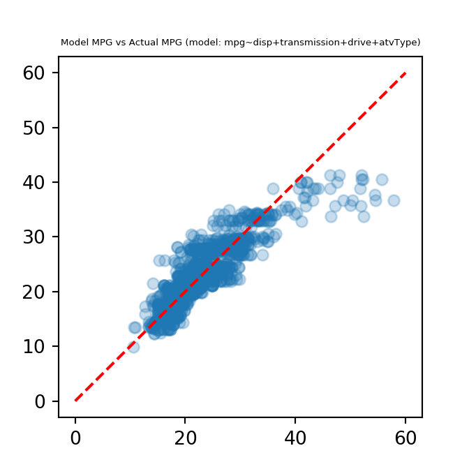

This model fits the training data more closely that the univariate model. In particular the vehicles with higher mpg are now closer to the diagonal line.

In future notebooks, I will utilise more of the functionality and methods available in scikit-learn.