This notebook is an example of using R to tackle a prediction problem using machine learning.
The aim is to fit a model that predicts a vehicle’s fuel efficiency - as measured in miles per gallon (MPG) - of vehicles, using the known values of other characteristics of the vehicle.
This particular example was most-immediately inspired by a case study in the excellent free online course Supervised Machine Learning Case Studies in R developed by Julia Silge. That case study involves 2018 model year vehicles, while this one uses 2020 model year vehicles. There are also multiple other similar data sets that are commonly used for case studies in regression.
Three types of models are calibrated in this notebook:
linear regression using Ordinary Least Squares (OLS)
decision trees
random forests
Reading in data
I have saved the data set used to a github repository. It can be read in using the following code:
cars2020 <- read.csv("https://raw.githubusercontent.com/thisisdaryn/data/master/ML/cars2020.csv") What does the data look like?
The input data consists of 1,164 observations of 14 variables that you can browse in the table below.
What does the data represent?
The columns in the data contain the following variables respectively:
make: brand of the vehiclemodel: name of a specific car productmpg, miles per gallon: a representative number for the number of miles the car can be driven while using 1 gallon of fueltransmission, Automatic, CVT, or Manualgears, number of gearsdrive, drivetrain: 4WD, AWD, FWD, PT 4WD, RWDdisp, engine displacement (in liters)cyl, number of cylindersclass, vehicle category: Compact, Large, Mid St Wagon, Midsize, Minicompact, Minivan, Sm Pickup Truck, Sm St Wagon, Sm SUV, SPV, Std Pickup Truck, Std SUV, Subcompact, or Two Seatersidi, Spark Ignited Direct Ignition: Y or Naspiration: Natural, Super Super+Turbo, Turbofuel, primary fuel type: Diesel, Mid, Premium, RegularatvType, alternative technology: Diesel, FFV, Hybrid, None, or Plug-in HybridstartStop, start-stop technology Y or N
The modeling Process
Splitting the data for training and testing
First, use the initial_split, training and testing functions of the rsample package, to split the data into disjoint sets for training and testing.
In particular, this code: * splits the data in a 80:20 ratio (training:testing). * uses the outcome variable, mpg to stratify. This is done to ensure that the distribution of the outcome is comparable in both data sets.
library(rsample)
set.seed(1729)
split <- initial_split(cars2020, prop = 0.8, strata = mpg)

train <- training(split)
test <- testing(split)
Checking the distribution of mpg in the training and tests
To visualize the distribution of the outcome, mpg, here is some code:
- Labeling each of the training and tests sets and then combining them for the purposes of making the plot:
library(dplyr)
cars_recon <- bind_rows(mutate(train, Data = "Training"),
mutate(test, Data = "Testing"))- Using
ggplot2to plot the density of the mpg variable:
library(ggplot2)

ggplot(cars_recon, aes(x = mpg, fill = Data)) +
  geom_density(alpha = 0.4)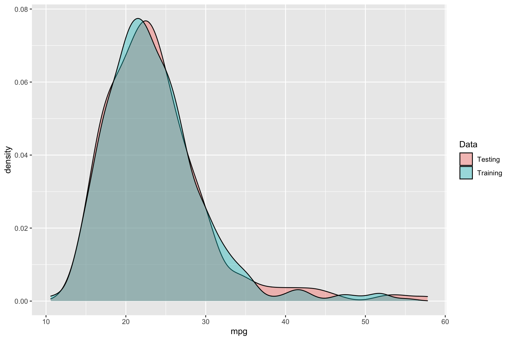
A note on Exploratory Data Analysis (EDA)
For the purpose of brevity I will skip the exploratory data analysis phase of the modeling process. All models calibrated in this notebook will use all available predictors other than make and model.
Removing ID variables
First remove the make and model variables.
id_cols <- c("make", "model")
train <- train[,!(names(train) %in% id_cols)]
Creating a linear model with Ordinary Least Squares
To fit a linear model using the method of Ordinary Least Squares (OLS) use the lm function. The . symbol in the formula/first input indicates that the model is to use all available predictors.
ols_model <- lm(mpg~., data = train)Click here for a model summary
summary(ols_model)
Call:
lm(formula = mpg ~ ., data = train)

Residuals:
    Min      1Q  Median      3Q     Max
-8.3468 -1.3866 -0.0745  1.4741 14.8510

Coefficients: (1 not defined because of singularities)
                      Estimate Std. Error t value Pr(>|t|)
(Intercept)           39.39621    1.02868  38.298  < 2e-16 ***
transmissionCVT        2.99197    0.38840   7.703 3.50e-14 ***
transmissionManual    -0.22690    0.26900  -0.843 0.399185
gears                 -0.33069    0.06699  -4.937 9.48e-07 ***
driveAWD               0.38524    0.30324   1.270 0.204271
driveFWD               3.71337    0.35806  10.371  < 2e-16 ***
drivePT 4WD            1.16997    0.62114   1.884 0.059943 .
driveRWD               1.24687    0.31581   3.948 8.49e-05 ***
disp                  -1.82473    0.25637  -7.118 2.25e-12 ***
cyl                   -0.53934    0.15724  -3.430 0.000631 ***
classLarge            -0.30636    0.41174  -0.744 0.457032
classMid St Wagon      0.19273    1.06990   0.180 0.857086
classMidsize           0.17684    0.35893   0.493 0.622353
classMinicompact      -1.47287    0.60084  -2.451 0.014422 *
classMinivan          -5.06545    1.02032  -4.965 8.24e-07 ***
classPassenger Van    -6.03105    2.06211  -2.925 0.003535 **
classSm Pickup Truck  -5.58664    0.74818  -7.467 1.94e-13 ***
classSm St Wagon       0.15969    0.61984   0.258 0.796744
classSm SUV           -2.91537    0.35774  -8.149 1.22e-15 ***
classSPV              -5.72648    0.69316  -8.261 5.13e-16 ***
classStd Pickup Truck -2.96265    0.52879  -5.603 2.81e-08 ***
classStd SUV          -2.96569    0.42871  -6.918 8.72e-12 ***
classSubcompact       -0.43112    0.40632  -1.061 0.288962
classTwo Seater       -0.95168    0.52976  -1.796 0.072760 .
sidiY                  0.73903    0.27948   2.644 0.008330 **
aspirationSuper       -1.59585    0.51935  -3.073 0.002185 **
aspirationSuper+Turbo -2.77630    1.59378  -1.742 0.081858 .
aspirationTurbo       -2.79223    0.29996  -9.309  < 2e-16 ***
fuelMid               -1.32542    1.29164  -1.026 0.305094
fuelPremium           -2.82644    0.95326  -2.965 0.003107 **
fuelRegular           -2.18991    0.96645  -2.266 0.023693 *
atvTypeFFV            -3.57468    0.89839  -3.979 7.48e-05 ***
atvTypeHybrid          2.07897    0.62508   3.326 0.000917 ***
atvTypeNone           -2.94116    0.56105  -5.242 1.98e-07 ***
atvTypePlug-in Hybrid       NA         NA      NA       NA
startStopY             1.60107    0.23586   6.788 2.06e-11 ***
---
Signif. codes:  0 '***' 0.001 '**' 0.01 '*' 0.05 '.' 0.1 ' ' 1

Residual standard error: 2.683 on 898 degrees of freedom
Multiple R-squared:  0.8258,    Adjusted R-squared:  0.8192
F-statistic: 125.2 on 34 and 898 DF,  p-value: < 2.2e-16
An alternative linear model (also with OLS)
I also, fit an alternative OLS model. This alternative model differs from the previous in using an outcome of \(log(mpg)\). This is done in following the example in the Case Study. This choice is suggested there because of the lognormal nature of the distribution of mpg values.
ols_log_model <- lm(log(mpg)~., data = train)Click here for a model summary of ols_log_model
summary(ols_log_model)
Call:
lm(formula = log(mpg) ~ ., data = train)

Residuals:
     Min       1Q   Median       3Q      Max
-0.32395 -0.05251 -0.00130  0.05891  0.34397

Coefficients: (1 not defined because of singularities)
                       Estimate Std. Error t value Pr(>|t|)
(Intercept)            3.825910   0.034847 109.792  < 2e-16 ***
transmissionCVT        0.105444   0.013157   8.014 3.44e-15 ***
transmissionManual    -0.018431   0.009113  -2.023 0.043416 *
gears                 -0.005682   0.002269  -2.504 0.012456 *
driveAWD               0.014536   0.010272   1.415 0.157404
driveFWD               0.126724   0.012129  10.448  < 2e-16 ***
drivePT 4WD            0.029596   0.021041   1.407 0.159894
driveRWD               0.051070   0.010698   4.774 2.11e-06 ***
disp                  -0.083764   0.008685  -9.645  < 2e-16 ***
cyl                   -0.030666   0.005327  -5.757 1.17e-08 ***
classLarge            -0.004605   0.013948  -0.330 0.741360
classMid St Wagon      0.009338   0.036243   0.258 0.796730
classMidsize           0.006892   0.012159   0.567 0.570975
classMinicompact      -0.048835   0.020354  -2.399 0.016628 *
classMinivan          -0.155215   0.034564  -4.491 8.02e-06 ***
classPassenger Van    -0.333828   0.069855  -4.779 2.06e-06 ***
classSm Pickup Truck  -0.222702   0.025345  -8.787  < 2e-16 ***
classSm St Wagon      -0.007791   0.020997  -0.371 0.710691
classSm SUV           -0.103913   0.012119  -8.575  < 2e-16 ***
classSPV              -0.238173   0.023481 -10.143  < 2e-16 ***
classStd Pickup Truck -0.116841   0.017913  -6.523 1.15e-10 ***
classStd SUV          -0.118853   0.014523  -8.184 9.35e-16 ***
classSubcompact       -0.009221   0.013764  -0.670 0.503088
classTwo Seater       -0.043939   0.017946  -2.448 0.014538 *
sidiY                  0.035687   0.009468   3.769 0.000174 ***
aspirationSuper       -0.080592   0.017593  -4.581 5.28e-06 ***
aspirationSuper+Turbo -0.125224   0.053990  -2.319 0.020596 *
aspirationTurbo       -0.115001   0.010161 -11.318  < 2e-16 ***
fuelMid               -0.076312   0.043755  -1.744 0.081484 .
fuelPremium           -0.157530   0.032292  -4.878 1.27e-06 ***
fuelRegular           -0.142901   0.032739  -4.365 1.42e-05 ***
atvTypeFFV            -0.097355   0.030433  -3.199 0.001428 **
atvTypeHybrid          0.057024   0.021175   2.693 0.007213 **
atvTypeNone           -0.088911   0.019006  -4.678 3.34e-06 ***
atvTypePlug-in Hybrid        NA         NA      NA       NA
startStopY             0.049559   0.007990   6.203 8.46e-10 ***
---
Signif. codes:  0 '***' 0.001 '**' 0.01 '*' 0.05 '.' 0.1 ' ' 1

Residual standard error: 0.09088 on 898 degrees of freedom
Multiple R-squared:  0.8697,    Adjusted R-squared:  0.8648
F-statistic: 176.3 on 34 and 898 DF,  p-value: < 2.2e-16
Decision Tree models
Next, we move on to fitting 2 decision tree models using the rpart package. Each decision tree model is formulated with an equivalent predictor to one of the OLS models
library(rpart)
dt_model <- rpart(mpg~., data = train)
dt_log_model <- rpart(log(mpg)~., data = train)
The decision tree formulated can be viewed using rpart.plot::rpart.plot:
library(rpart.plot)
rpart.plot(dt_model)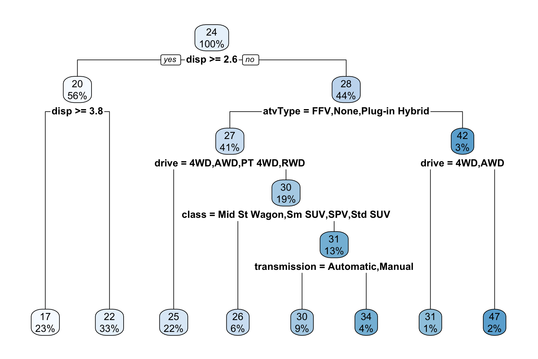
Click here for a visualization of the dt_log_model
rpart.plot(dt_log_model)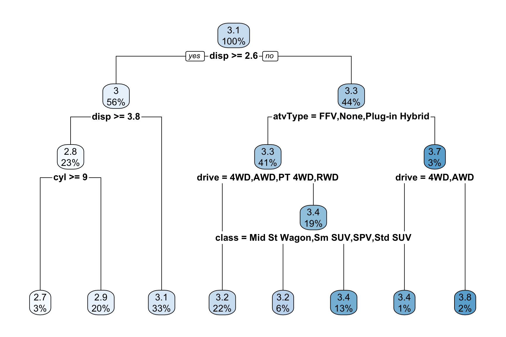
Random Forest models
Last, formulate two random forest models (one for each of the predictors):
library(randomForest)
set.seed(2001)
rf_model <- randomForest(mpg~., data = train)
set.seed(99)
rf_log_model <- randomForest(log(mpg)~., data = train)
Collating model estimates
Now that all 6 models have been formulated, I use dplyr::mutate to add the model estimates to a data frame that also contains the actual mpg values as well as the model predictors.
train_results <- mutate(train,
                        ols = predict(ols_model, train),
                        ols_log = exp(predict(ols_log_model, train)),
                        dt = predict(dt_model, train),
                        dt_log  = exp(predict(dt_log_model, train)),
                        rf = predict(rf_model, train),
                        rf_log = exp(predict(rf_log_model, train))
                        )
Here, I got a warning prediction from a rank-deficient fit may be misleading after each call to randomForest. (I’m ignoring them for now.)
Visualizing model performance
Now, to visualize the model performance by graphing the model estimates vs the corresponding actual values of the fuel efficiency.
The code below uses tidyr::pivot_longer to reshape the data to be used easily with ggplot2 subsequently.
library(tidyr)
train_results_long <- pivot_longer(train_results, ols:rf_log,
                                   names_to = "method", values_to = "estimate") %>%
  select(mpg, method, estimate)
head(train_results_long)
# A tibble: 6 x 3
mpg method estimate
<dbl> <chr> <dbl>
1 27.9 ols 28.7
2 27.9 ols_log 28.6
3 27.9 dt 29.7
4 27.9 dt_log 30.9
5 27.9 rf 27.6
6 27.9 rf_log 27.5Now make a faceted plot of the model estimates vs the actual MPG values using ggplot2:
ggplot(data = train_results_long,
       aes(x = mpg, y = estimate)) +
  geom_point(shape = 21, colour = "blue") + facet_wrap(~method, ncol = 2) +
  geom_abline(slope = 1, intercept = 0)   +
  xlim(c(0,60)) + ylim(c(0,60)) + theme_minimal()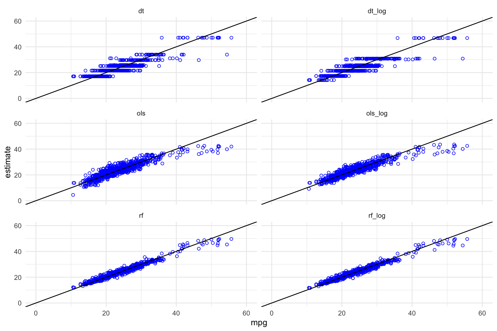
Points on the diagonal line correspond to cars for which the model estimated value and the actual mpg value are very close. Points that are above or below the line correspond to cars for which the model overestimates or underestimates the mpg respectively.
Inspecting these plots visually, it seems to me that the random forest models fit more closely than the OLS models, which fit more closely than the decision tree models.
Getting model metrics
The yardstick::metrics function can be used for summary statistics for a model. It requires that the model estimates be available in as a column of a data frame that also contains a column of corresponding truth values.
library(yardstick)

metrics(train_results, truth = mpg, estimate = ols)
# A tibble: 3 x 3
.metric .estimator .estimate
<chr> <chr> <dbl>
1 rmse standard 2.63
2 rsq standard 0.826
3 mae standard 1.91 The three reported metrics are:
Root mean squared error
\(R^2\)
Mean absolute error
Comparing models using RMSE
Next, I wrote some code that would compare multiple models using a specified metric.
The comp_models function takes the following inputs:
* A data frame containing the truth values as well as a column with the estimates of each model
* the names of the columns corresponding to model estimates
* the name of the column with the true outcome values
* the chosen metric
metrics2 <- function(fit_name, in_df, truth){
  out_df <- yardstick::metrics(in_df, fit_name, truth)
  out_df$fit <- fit_name
  return(out_df)
}
comp_models <- function(in_df, fit_names, in_truth, metric, prefix = ""){

  out_df <- purrr::map_df(fit_names, metrics2, in_df = in_df, truth = in_truth)
  out_df <- out_df %>% filter(.metric == metric) %>%
    select(fit, .estimate) %>% arrange(.estimate)
  names(out_df)[2] <- paste(prefix, metric)
  return(out_df)
}
Now we can use comp_models to get the rmse for each of the models fitting on the training data:
model_names <- c("ols", "ols_log", "dt", "dt_log", "rf", "rf_log")
train_rmse <- comp_models(train_results,
                          model_names,
                          in_truth = "mpg",
                          metric = "rmse",
                          prefix = "train")

train_rmse
# A tibble: 6 x 2
fit `train rmse`
<chr> <dbl>
1 rf 1.25
2 rf_log 1.26
3 ols_log 2.35
4 ols 2.63
5 dt 2.75
6 dt_log 2.81This gives an ordering of the closeness of the fit using the selected metric.
Evaluating model performance on the testing data
Now to test how the models do on the unseen testing data. I use similar code as before to augment the testing data frame with the model estimates for each of the 6 models:
test_results <- mutate(test, ols = predict(ols_model, test),
                       ols_log = exp(predict(ols_log_model, test)),
                       dt = predict(dt_model, test),
                       dt_log  = exp(predict(dt_log_model, test)),
                       rf = predict(rf_model, test),
                       rf_log = exp(predict(rf_log_model, test))
)
Visualizing model performance on the testing data
And now to visualize the model estimates vs actual MPG values in a similar manner to what was done previously:
test_results_long <- pivot_longer(test_results,
                                  ols:rf_log,
                                  names_to = "method",
                                  values_to = "estimate")

ggplot(data = test_results_long,
       aes(x = mpg, y = estimate)) +
  geom_point(shape = 21, colour = "blue") +
  facet_wrap(~method, ncol = 2) +
  geom_abline(slope = 1, intercept = 0) +
  xlim(c(0,50)) + ylim(c(0,50)) +
  theme_minimal()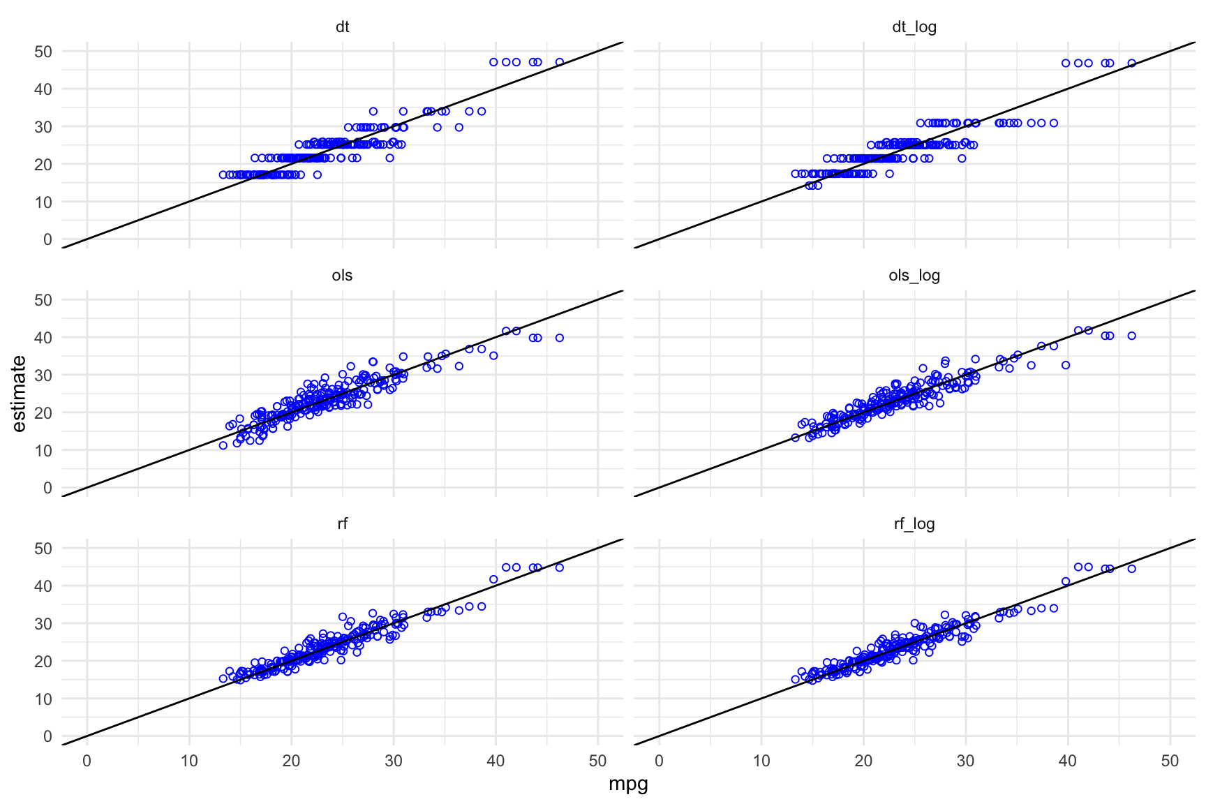
Comparing model performance on test data using RMSE
And a comparison of RMSE values for each of the models:
test_rmse <- comp_models(test_results,
                         model_names,
                         in_truth = "mpg",
                         metric = "rmse",
                         prefix = "test")

test_rmse
# A tibble: 6 x 2
fit `test rmse`
<chr> <dbl>
1 rf 2.00
2 rf_log 2.02
3 ols_log 2.79
4 dt 2.90
5 dt_log 2.94
6 ols 3.04The rankings of the models - as measured by RMSE - has changed. Specifically, the first model ols has not generalised to the testing data set as well as the other models.
I also used dplyr::inner_join to see how the RMSE values changed collectively moving the models from the training data to the testing data.
inner_join(train_rmse, test_rmse, by = "fit")# A tibble: 6 x 3
fit `train rmse` `test rmse`
<chr> <dbl> <dbl>
1 rf 1.25 2.00
2 rf_log 1.26 2.02
3 ols_log 2.35 2.79
4 ols 2.63 3.04
5 dt 2.75 2.90
6 dt_log 2.81 2.94This is the end of this notebook. Feel free to send feedback to thisisdaryn at gmail dot com.